Tricubic spline interpolants

I wanted a straightforward, easy-to-install, and fast way of calculating tricubic interpolants on a three dimensional regular grid in Python and set out to do it myself. I extended the original code in C to be accessible by numpy using f2py, and it can compete or beat the equivalent bicubic interpolating splines in scipy in speed (in some cases). The increased speed came through the addition of a finite difference matrix and by intelligently reusing spline coefficients.

This required the following:

• An easy object-oriented interface
• Inclusion of finite differences and sorting
• Interfacing with f2py
• Managing boundary conditions

While there are implementations of tricubic interpolation in a number of languages (including java, C++ and Python), there was not one that matched all of these requirements. In taking on this project, it became clear that this task was actually more difficult that I had originally imagined, first off the original work by Lekien and Marsden did not include the matrix needed for calculating the interpolation coefficients in the paper (as it is a 64x64 matrix) and the linked website containing the matrix no longer exists (though someone seems to have found a version and pushed it to Github). After finding it after some searching, I went to work.

My version builds directly from Lekien and Marsden’s original, adding and streamlining the interpolation. In this way this work is not something groundbreaking. However, I extend it by making it more user friendly so that it can work with vector and arrays, by iterating through the evaluation in a somewhat intelligent way, and speeding the derivative calculations for a regular grid by including a finite difference matrix in the spline coefficient generating matrix (removing all need for calculating derivatives). Finally, I make it easily accessible to a scripting language. All of these additions successfully contribute in making it simpler and faster to use.

The reason why its written in C is three-fold. First, the original was written in C and was a good starting point (allowing for progressive debugging of the output to compare against the original). Secondly and most importantly the code needed to be fast enough to compete with other two-dimensional interpolators. Serious time and effort by many programmers and mathematicians have gone into making extremely fast 2D interpolating schemes in base lower-level languages (e.g. FORTRAN, C and C++). It was my hope to be somewhere in a similar ballpark in speed even though I knew the amount of computation for tricubic interpolation would be greater. Thirdly, C and Python can be directly and natively interfaced easily through the ctypes package and through f2py (part of numpy). This would allow for direct access with Python (also reducing the barrier for its use).

Dependency can be your enemy

One things that bugs me a lot are software packages which require a lot of other programs to be installed to operate. When working on a stable system which is relatively common (like a standard architecture computer with a reasonable operating system) there are usually no problems. Most of the time you can even get a precompiled binary. But if you go to a rarer system type, whether its Solaris, a weird Linux distro or an older PowerPC computer, the higher the probability you will run into an issue and you will have to install by hand. The operation and installation of your software is now determined by the operability and install-ability of someone else’s work. The weak link in the robustness of your software moves into a distinct region of ‘unknown unknowns’ where you don’t know what the problems might be or how to solve them ( i.e. someone else’s problem is now your problem). Nothing annoys me more than trying to solve a clash between source code and a specific architecture for code I haven’t written. In this way dependency of code can really be an enemy.

It is my opinion that widely distributed code should be written to depend on as few packages as possible and it should focus on only using dependable, common and vetted software to build from. The more mainstream the package, the more likely that there is someone else who has already faced the problem and solved it (super important for Solaris and stackoverflow).

On the other hand, there is something to be said for not ‘reinventing the wheel’. For example, you will never beat BLAS/ATLAS at doing matrix methods, so there is no reason do your own QR decomposition algorithm. However, in any case that you do find a ‘plug and play’ solution in another software package, ask yourself if it is worth it. The answer can be highly contextual too: if it is personal scripting for a specific problem then installing the package and using it is probably a good idea. If you want some code for others to routinely use for an indeterminate amount of time, its probably a bad choice. However, if it is standardized and ubiquitous to the point of trivial availability, then this discussion points towards using that code. (For Solaris you’d be surprized, I had to once build LAPACK and BLAS from scratch).

This long-winded philosophical diatribe is a motivation for the use of f2py. f2py is a program which can compile FORTRAN and C code for use in numpy/Python. Numpy is very commonly installed with Python for scientific computing. In this case, I knew that others would be using my software on any number of operating systems and computers. Therefore by having it only depend on one code on top of Python and having this dependency being extremely common would greatly simplify installation and debugging. This interfacing code is utilized extensively for giving Python some ‘speed’ by relying on the underlying speed of FORTRAN.

f2py and C is less common, but there are guides. The only additional file necessary is a .pyf file which provides the necessary ‘glue’ for f2py to work.

    
       f2py -c _tricub.pyf _tricub.c
    
  

This is all that is needed to compile my code for use. It even works easily with setup.py and pip installs. Again, it is super easy entry for a non-developer to use. It generates a .dll file in Windows or a .so file on UNIX systems, which is then easily accessible by Python and other codes for use. This is a similar approach utilized by scipy and numpy for optimized routines.

Simple optimizations for regular grids

The work by Lekien and Marsden was generalized to interpolate the value of a point within any voxel where certain values at the vertices are known (in a cartilinear geometry). This means that the original code requires the input of various derivatives at the corners of the voxel and as a consequence these values need to be generated ahead of time. Most, if not all current implementations of the Lekien and Marsden algorithm use a separate step for the generation of the necessary derivatives. Derivatives represent 56 of the 64 needed values, and these 56 values are generated from finite differences. These values create a 64x1 vector $v$ which is multiplied by 64x64 matrix given by Lekien and Marsden known as $A^{-1}$. This calculated yields the necessary coefficients to the various cubic polynomials $p$.

$$p = A^{-1} \cdot v$$

In the case of a regular grid, a finite difference matrix can be used to reduce the necessary calculations necessary for the interpolation. The generation of the $v$ vector is a simple 64x64 matrix multiplication dependent on the surrounding 3x3x3 grid of voxels (4x4x4 grid of vertices). The values of these vertices are given by $x$. Generating the coefficients $p$ takes the following form (if $B$ is finite difference matrix):

$$p = A^{-1} \cdot ( B \cdot x )$$

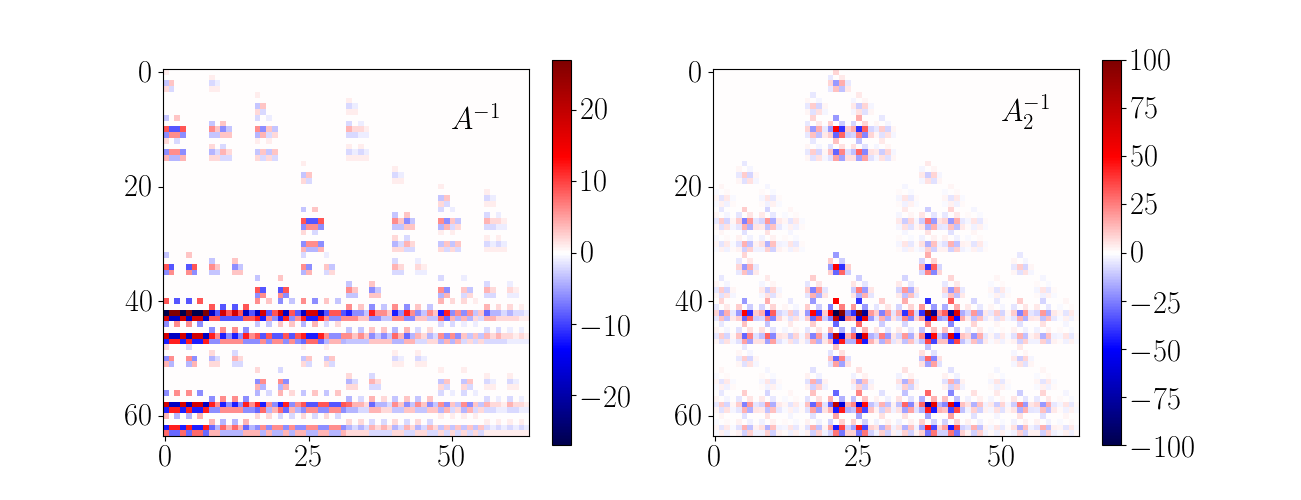
The associative property of matrix multiplication allows for the definition of a new matrix $A^{-1}_2 = A^{-1} \cdot B$. This combined matrix removes all necessary calculation of derivatives by incorporating them in the matrix multiplication needed to form the polynomial coefficients; this new matrix is defined as $A_2^{-1}$. Essentially, the mathematical difficulty in generating $A_2^{-1}$ removes the work necessary in the numerical calculation of the derivatives. (However, in practice $A_2^{-1}$ is an integer matrix, and requires a division by 8 to yield the correct values.)

$A_2^{-1}$ is defined for a specific ordering of the 3x3x3 voxel matrix, and can be readily redefined for different ordering schemes. In my definition I assumed that the axis `closest’ in memory is dominant with a hierarchical scheme similar for the other two axes. These seemed to be the most straightforward. It should be noted however that a specific ordering of the vertices is expected in the $x$ vector.

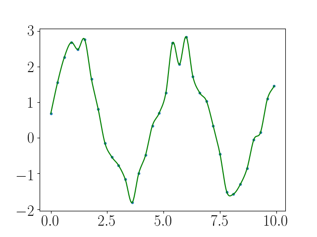
A second way of quickly reducing computation is to not calculate them more than once. Reusing coefficients after their initial calculation greatly reduces the necessary derivation by reducing the number of redundant calculations. On a regular grid, it is straightforward to find, sort, and group the various points into specific voxels using standardized C sort functions.

Once the coefficients are derived for a specific voxel, the interpolated value is simply an iteration and summation over the polynomials. The increased computation in sorting and grouping the interpolation points is greatly offset by the reduced number of matrix multiplications. However, this is dependent on the number and grouping of points needed to interpolated.

Pesky edges and Neumann boundary conditions

In nearly all implementations of the Leiken and Marsden tricubic interpolation, it is assumed that all the necessary derivatives can be easily calculated from the input data arrays. Similarly, the regular grid implementation use of $A_2^{-1}$ contains the same assumption. However, when an interpolation point is beside the edge of the data grid (in any or all of the grid directions) the needed 3x3x3 voxel group needed for finite differencing cannot be generated. Similar issues exist for cubic and bicubic splines when interpolation occurs close to the boundaries. Schemes for interpolation near the borders of those splines can be extended to tricbuic splines. These schemes make assumptions about the nature of the missing data, specifically about the nature of the edge gradients (derivatives). A Neumann boundary condition solution was implemented in this Tricubic interpolation implementation in order to guarantee operability of the code within the entirety of the defined grid.

The simplest and most straightforward approach when data is not available is to assume that the derivatives at the edge conditions are zero. The easiest way to implement this Neumann condition within the $A_2^{-1}$ framework is to pad the grid with additional data at the edges. This data merely replicates the value at the edges and allows for the original algorithm of to be utilized. In the implemented script the padding of the data with two additional values in all directions originally occurred within the initialization of the Python object, but later iterations moved it to the C implementation. This isolates the necessary computation within a single language in the case that other languages which to interface with the underlying C.

Other more complicated (and possibly more accurate) methods exist for generating the edge derivatives yielding more `natural’ and possibly accurate solutions. However, I decided that the cost in time for implementing those solutions would be not worth the effort, as well-conditioned reproductions with splines truly requires higher fidelity data by users. If the derivatives near the edge are not well-conditioned, then the entire problem may instead be ill-posed. This simple, quick solution was only meant to yield plausibly accurate solutions in the cases where the entire grid is naively interpolated upon.

Putting it all together

The tricubic interpolation algorithm is included in the Eqtools package. This package is meant to map and characterize two dimensional tokamak coordinate systems (a type of toroidally symmetric magnetic fusion power device) called equilibria. This mapping utilizes interpolation on a two dimensional grid to determine the a value which is converted into another coordinate system of interest. Often, multiple two dimensional grids are available at various times creating a time evolution of a tokamak plasma. In normal implementations, the mapping of a point occurs in the grid nearest in time. This creates discontinuities which can affect time-dependent phenomenon.

The time dependent data is three-dimensional and can also now be spline interpolated in time, providing continuous and smooth solutions. This was put on display in the publication which first described the Eqtools package. In it, several calculated equilibria are dramatically over a time series. The shape of surfaces of the plasma within the tokamak are shown in shades of blue. The 3D data given by the nearest neighbor interpolation is rough in time with many discontinuities. However, the tricubic interpolation example has smooth variation.

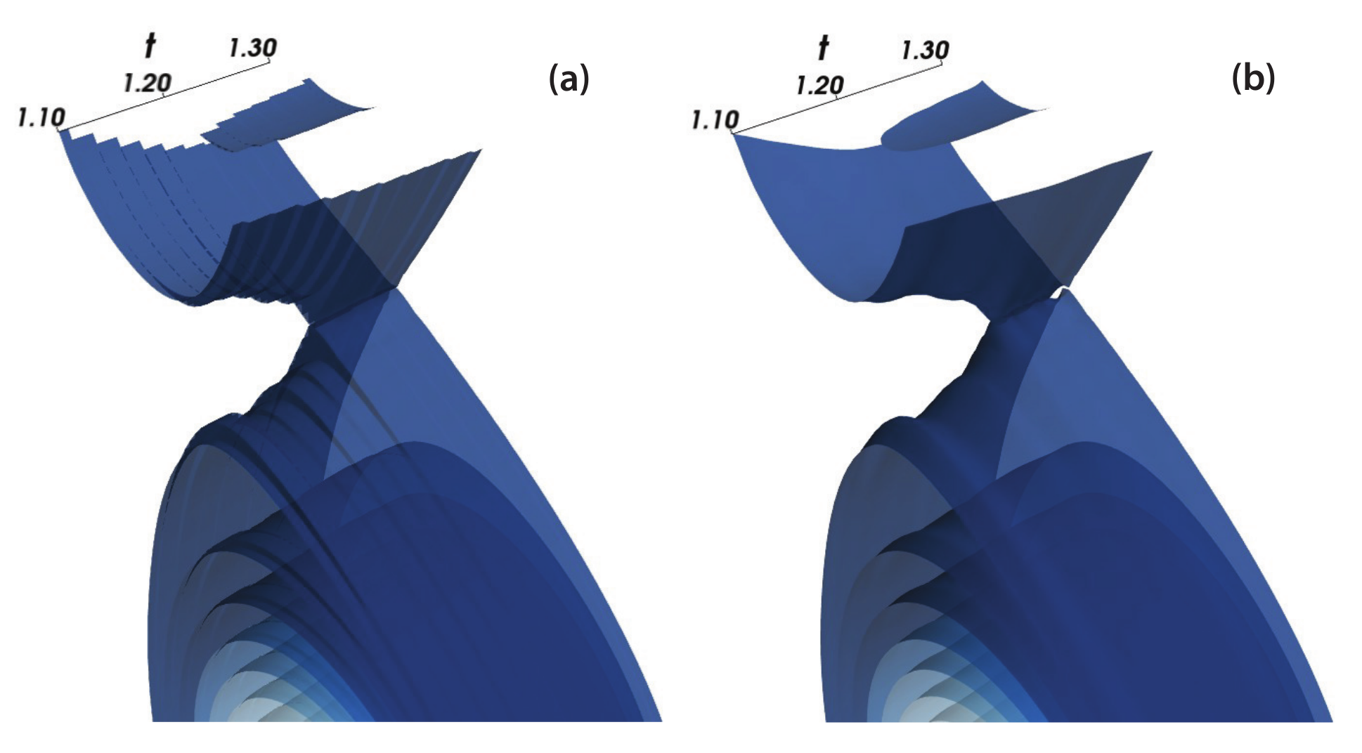
This shows the power of such tricubic interpolation in the right circumstances. In naturally regular data sets (where all three axes are consistent), the implementation is extremely useful. There are other similar data sets which could utilize such a system, such as for ethereal data like smoke, or weather data. In total, this project was useful for trying to bring tricubic interpolation more mainstream utilization.

You can find the implementation at the following link: Eqtools

The paper which describes the additions to the original implementation: Paper