In honor of some of my colorblind students at MIT, I wrote a code which can generate an Ishihara test from sets of simply-connected polygons. The outcome is a working example of the ‘Beast’ hall symbol.
This required the following:
- Monte Carlo circle placement
- Algorithm for line-circle intersections
- Algorithm for if a point is within a polygon
- Extraction of polygon vertices from the svg format
- Proper coloring for the colorblind
Monte Carlo circle placement
The Ishihara test attempts to obfuscate an object through the use of randomly-placed, differently-sized circles. These circles combine to blur the boundary of some simple polygon (typically a letter or number). Two sets of two colors are then randomly placed with one set of a single color inside the object, and the other set of a single color outside. Usually this is a dark and light red, and then a dark and light green. Together the random blotches of colors and circles transforms the original object into something difficult to determine for someone who is colorblind. Yet the separation of the color sets allows for the objects to be easily identified for those with normal vision. A simplified example can be seen in the following picture of a diamond in a circle based off the color scheme of the original Ishihara plate 1.
Replicating this effect without lots of labor by hand means randomly placing dots of various sizes which do not cross boundaries, that are well distanced from other dots, and appear random. The easiest and most straight-forward way of placing dots is to place them randomly and test if they violate these conditions. This simple Monte Carlo method rests on being able to create an array of valid dots and polygon lines which are compared to the next random dot. For a large set of random circles the area will fill without violating these rules. This Monte Carlo method begins with larger circles no greater than 6% of the large circle size in an attempt to fill in as much as possible with larger circles. Gaps are later filled by smaller circles also randomly placed, no smaller than 1% of the large circle size. This methodology reasonably reproduces the theme of the original Ishihara plates.
Line-circle intersections
The first problem is finding if the randomly placed circles cross the boundary of an object. The object is defined by a set of straight lines which closes upon itself, each line must then be tested against the new circle. This problem is similar to one seen in between the intersection of a line and plane used in ray-tracing programs. Solving for the intersection of a line and plane is a straightforward 3x3 matrix inversion. In two dimensions it is the intersection of two lines. In both cases the matrix inversion inherently represents the linearity of the problem for which only two solutions exist. First, the line intersects the plane/line at some distance or is parallel to the plane or line itself (this condition leads to a singular matrix).
Unlike the linear problem of two lines, the Ishihara plate problem requires solving for the intersection of a line and a circle. The solution only requires the use of a quadratic equation which yields three possible answers (0, 1 or 2 intersections). Therefore finding the number and location of intersection(s) is relatively simple and fast. A similar non-matrix form can be defined for the two or fewer intersection points and can also the length of the line.
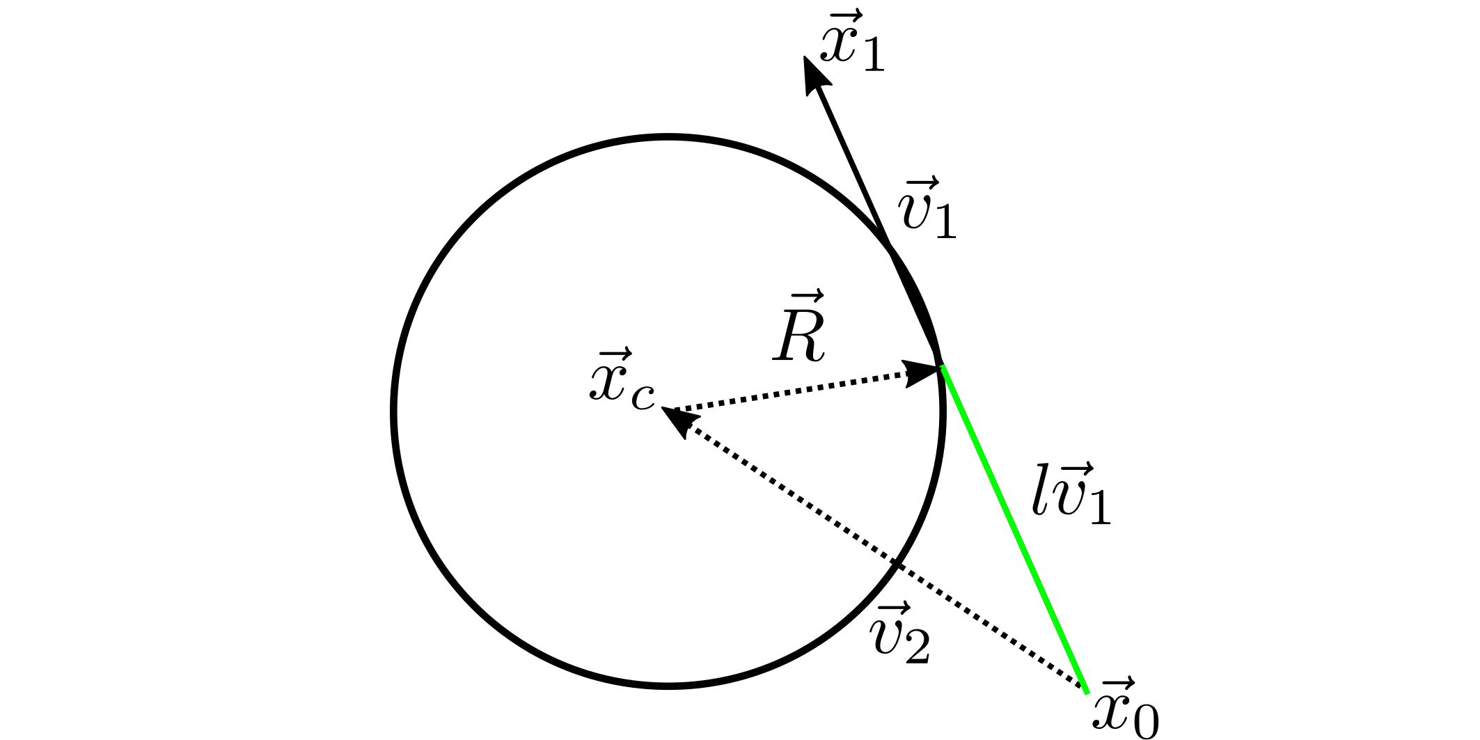
The center and radius of the circle is defined as the vector and respectively, and the endpoints of the two lines as vectors and . With , and a vector , the distance along (defined as ) of the intersection with the circle can be readily solved. The intersection of the circle and the occurs when a triangle is created with sides , , and . can be defined from a vector subraction and a dot product with itself.
Astute people will notice the second equation is the vector form of the law of cosines. This equation is quadratic in and can be readily solved for. If any solution with the value of is less than one, or if either or both points are within the circle (i.e. or ) the circle is removed. This test must be ran for every line which defines the object. An easier proceedure exists to compare the set of ‘good’ circles, by comparing the distance between centers to the sum of the two radii and some minimum separation distance , . Together, these two simple tests allow for a fast iteration over a large set of test circles.
How to tell if a circle is within an object
Once a valid circle is added to the set of other valid circles, the region of the circle needs to be determined for its coloring. Luckily this is a solved problem, with many available versions in many different codes. The problem is known as the ‘point in polygon’ problem. The essence of the solution is starting from the point, drawing a line to infinity, and counting the number of times it crosses the boundary of the object. If the total is even, it is outside and vice versa. A much more rigorous theorem associated with it known as the Jordan curve theorem. Rather than regurgitate the contents of other websites, its better to click these links and see the other (better) explanations. My friend had written a simple python program called inPolygon (there is a widely known MATLAB program with the same name and function) which we had used in a collaborative code and I simply reused it.
For each circle, a set of booleans is stored which describes if the circle is within a specific object. A specific logical statement can determine the necessary color set to use to match the original vector graphic. In the case of a two-color vector graphic the color can be set by the number of nested objects the circle is in ( i.e. if it is in an even or odd number of polygons).
Getting points out of an SVG file
An SVG file is a specially formatted XML document which can be parsed into a vector graphic. The outline of most objects in this format is defined by a ‘path’ tag. A ‘path’ contains a representative Bezier curve, spline or line. As higher order curves (e.g. parabolas and splines) require higher order root solving (cubic or quartic root) to find the intersection with circles, the goal is to reduce the vector graphic to straight lines. This simplification only requires extracting the endpoints which I assume are the vertices. The start and end points of every separate curve in a path is extracted and stored in a separate file as an array. Thus it is important to reduce said SVG picture to a sufficient number of straight-line segments which accurately reflect the image.
It was easier for a limited number of SVGs (or a simple shape) to extract the paths via the native python xml interface and the judicious use of string parsing to yield the end points. The points of the vertices are not large in number, and can be convieniently stored as a python pickle file.
A good guide to SVG file paths: https://developer.mozilla.org/en-US/docs/Web/SVG/Tutorial/Paths
A really useful stack overflow post: http://stackoverflow.com/questions/15857818/python-svg-parser
Putting it all together
Now that there is a methodology for generating the dots, testing them, and separating them in the proper groups, what colors should we use? Since I am not colorblind myself, the easiest solution is to extract colors from a true Ishihara plate and use those. From asking my students, the hardest to discern were using a dark and light color of red and of green. The hex colors I used were:
- Dark Red - #c1152d
- Light Red - #e2644e
- Dark Green - #008d37
- Light Green - #7cbc4a
Each dot was randomly assigned to be light or dark and given red or green based off of what polygon it was in. I tested a number of random dark/light distributions in order to make it as hard to see as possible (thanks to my ‘test-subjects’). The original image is a black and white of silhouette infront of a moon.
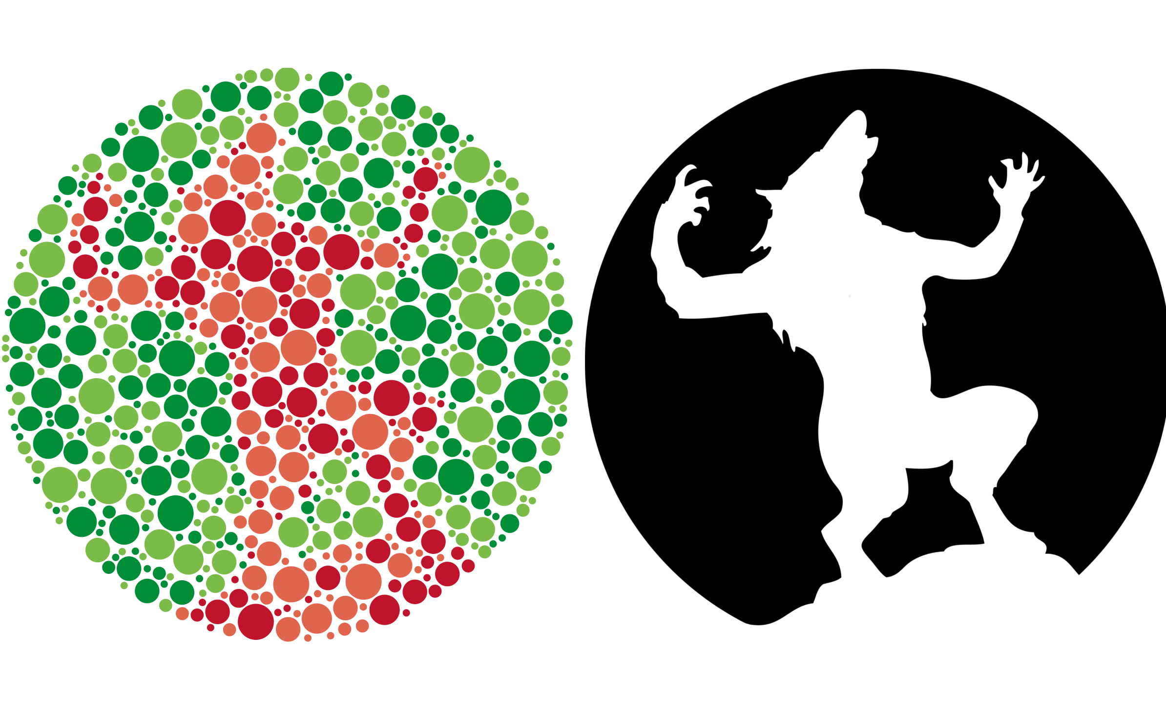
The more complicated the polygon path, the more difficult it is to mask the outline. While a diamond can be easy to mask, a 7 or 20 pointed star might be more difficult. At some point, jagged edges will only be filled by smaller circles to a point that they cannot be filled at all. This is becomes apparent in the circle structure around the hands and mouth, where large direction changes over small distances make for large gaps and small circles. This concept is related to something in optics and engineering known as ‘spatial frequency’ , which describes the variation in structure of an object space.
Taking the Fourier transform of the fingers, mouth and ears in space will yield indications of this effect (I believe). These parts are representative of strong high spatial-frequency effects which impact the ability to generate passable Ishihara plates. While I believe my example came out fine, I would caution against replicating pictures as Ishihara plates which are very detailed. Overall, the concepts of this project were rather straightforward, and the example code I used can be found here in my project Github repository.